
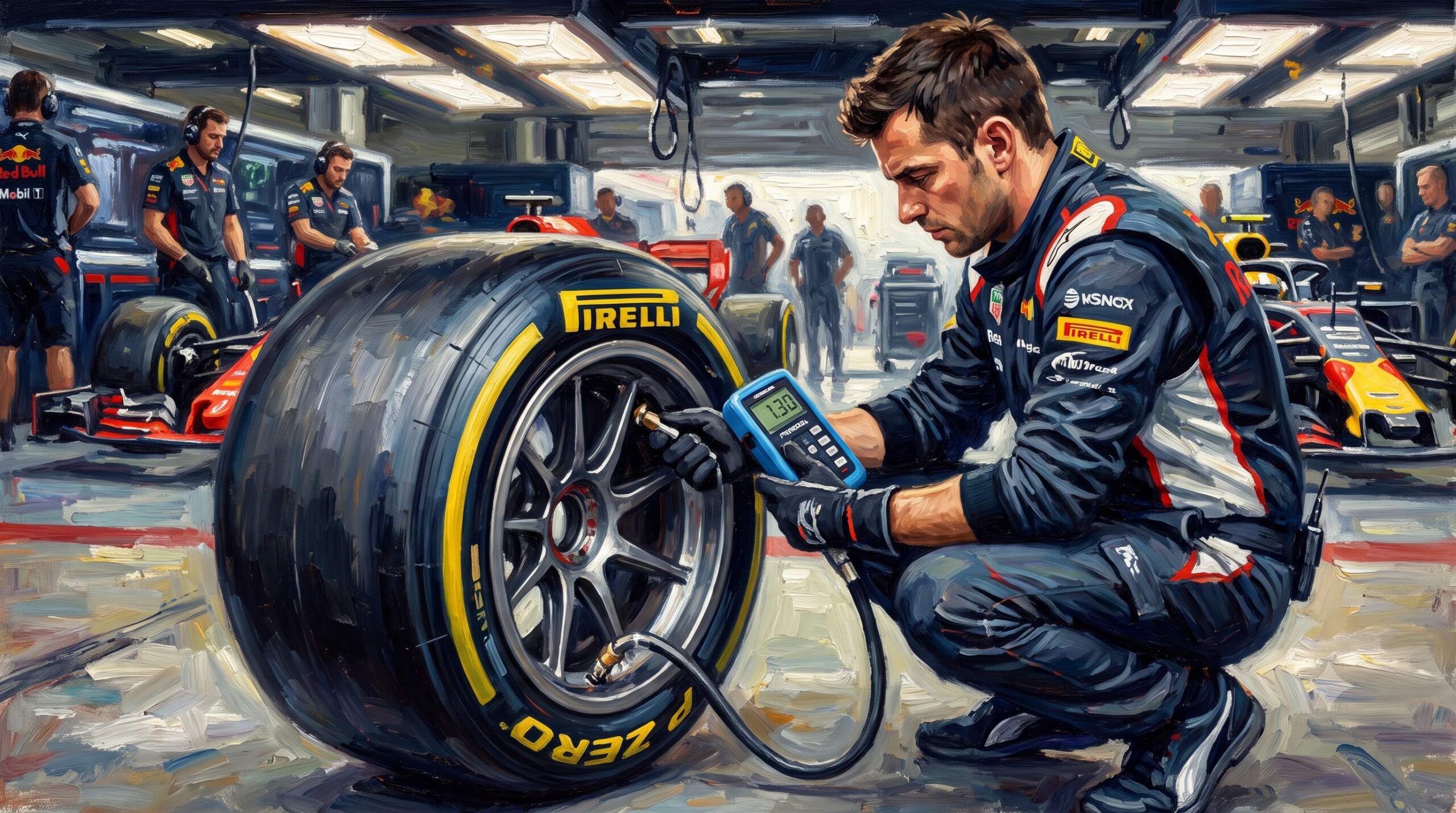
Finding the sweet spot for tire pressures is one of the most critical engineering challenges in Formula 1. At a historic and punishing circuit like the Circuit de Monaco—spanning 3,337 meters with 19 tight corners and virtually no breathing room—every millisecond counts. To crack this problem, we built a Python simulation model capturing the delicate balance between cornering grip and straightaway speed, testing how intelligent optimization can dramatically outperform brute-force methods.
Inside the Python Simulation
The core of our script rests on a custom lap simulator (simulate_lap) that accounts for the harsh realities of a 798 kg Formula 1 car navigating Monaco’s unique layout. Key physical layers modeled in the code include:
- Dynamic Thermal Expansion: Unlike static models, our thermal framework simulates how lower starting (cold) pressures cause aggressive sidewall flexing under load, generating internal friction and higher heat build-up.
- Lateral Grip: Governs cornering performance, mapping hot operating pressures against an optimal grip curve.
- Rolling Resistance: Simulates straightaway acceleration where tire pressures introduce drag penalties against the car’s 1,000-horsepower power unit.
Brute Force vs. Intelligence: Random Search vs. Bayesian Optimization
Initially, the script relied on a standard random search loop to sample cold pressures across legal Pirelli minimum boundaries. While a random search loop can eventually unearth decent configurations given enough time, it lacks directional memory. Granted, the random search loop would have improved significantly with 2,000 more epochs, but it remains a brute-force approach that is heavily prone to boundary traps and computational inefficiency.
To streamline this, we upgraded the optimization architecture to use Bayesian Optimization via the scikit-optimize library (gp_minimize). Instead of blindly guessing, Bayesian optimization builds a probabilistic Gaussian Process surrogate model of the simulation function. It smartly balances exploration by testing unknown pressure ranges with exploitation by honing in on promising regions.
The performance gains were striking. While the random search struggled to find a balanced optimum without exhaustive runs, gp_minimize systematically converged on an optimal setup in just 50 function calls, yielding a slick simulated lap time of 66.596 seconds with optimized cold pressures of 19.51 PSI (front) and 18.07 PSI (rear).
What Lies Ahead
By moving from raw stochastic guessing to smart probabilistic modeling, our Monaco simulation has transformed into a powerful engineering workbench. In the next article, I’ll explore aid* and add competing vehicles to the equation.
Formulas
Aerodynamic Drag: Uses the standard drag equation ($F_d = frac{1}{2} rho C_d A v^2$). The coefficient/area product ($C_d A = 1.85$) is appropriately high for a high-downforce Monaco setup.
Power-Limited Thrust: Approximates thrust force using power divided by velocity ($F = frac{P}{v}$), bounded by max(v, 1.0) to avoid division-by-zero singularities at rest.
Newton’s Second Law: $a = frac{F_{net}}{m}$ used correctly within an Euler integration loop ($v_{new} = v_{old} + a cdot dt$).
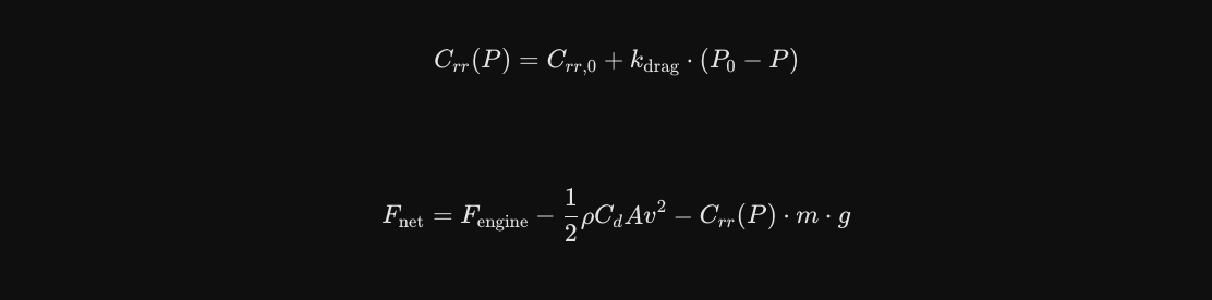
1) Rolling Resistance Coefficient
2) Net Force Equation
3) Tire Friction Coefficient
4) Maximum Cornering Velocity
Python Code
					import numpy as np
from skopt import gp_minimize
from skopt.space import Real
# ---------------------------------------------------------
# 1. CIRCUIT DE MONACO TRACK DEFINITION
# ---------------------------------------------------------
# Total official distance: precisely 3,337 meters
# Format: (length_in_meters, radius_in_meters) - radius 0 denotes a straight line
TRACK_SEGMENTS = [
    (210, 0),    # Pit Straight / Run to Turn 1
    (40, 28),    # Turn 1: Sainte Dévote (Tight right-hander)
    (420, 0),    # Turn 2: Beau Rivage (Uphill full-throttle sweep)
    (60, 65),    # Turn 3: Massenet (Long sweeping left)
    (45, 40),    # Turn 4: Casino Square
    (140, 0),    # Run down to Mirabeau Haute
    (35, 22),    # Turn 5: Mirabeau Haute
    (70, 0),     # Short downhill descent
    (35, 12),    # Turn 6: Grand Hôtel Hairpin (Slowest corner in F1, ~48 km/h)
    (60, 0),     # Descent to Mirabeau Bas
    (35, 22),    # Turn 7: Mirabeau Bas
    (50, 0),     # Short run to Portier
    (35, 20),    # Turn 8: Portier (Critical exit before the tunnel)
    (510, 280),  # Turn 9: The Tunnel (High-speed sweep, taken flat out at ~260 km/h)
    (110, 0),    # Heavy braking zone out of the tunnel
    (60, 18),    # Turn 10/11: Nouvelle Chicane
    (140, 0),    # Short run along the harbor
    (45, 55),    # Turn 12: Tabac (Fast left-hander)
    (90, 0),     # Approach to Swimming Pool
    (60, 48),    # Turn 13/14: Louis Chiron (Fast Swimming Pool entry chicane)
    (70, 0),     # Short run between chicane sections
    (50, 25),    # Turn 15/16: Swimming Pool exit chicane (Bumpy, tight exit)
    (110, 0),    # Run to La Rascasse
    (40, 14),    # Turn 17: La Rascasse (Very tight right-hand hairpin)
    (50, 0),     # Short approach to final corner
    (35, 22),    # Turn 18: Antony Noghès (Final corner before straight)
    (337, 0)     # Main Straight to finish line
]
# ---------------------------------------------------------
# 2. VEHICLE & TRACK SIMULATOR (MONACO AERO SETUP)
# ---------------------------------------------------------
def simulate_lap(psi_front, psi_rear):
    """
    Simulates a lap of Circuit de Monaco and returns total lap time in seconds.
    psi_front and psi_rear represent starting (cold) garage pressures.
    """
    mass = 798.0           # F1 car minimum weight in kg
    cd_area = 1.85         # Higher drag area due to high-downforce Monaco aero kit
    air_density = 1.225
    power = 745000.0       # ~1000 hp in Watts
    g = 9.81
    # --- DYNAMIC THERMAL EXPANSION MODEL ---
    base_boost_front = 2.0
    base_boost_rear  = 2.5
    flex_sensitivity = 0.20
    heat_boost_front = base_boost_front + flex_sensitivity * max(0.0, 22.0 - psi_front)
    heat_boost_rear  = base_boost_rear  + flex_sensitivity * max(0.0, 20.0 - psi_rear)
    hot_psi_front = psi_front + heat_boost_front
    hot_psi_rear  = psi_rear  + heat_boost_rear
    # 1. LATERAL GRIP
    mu_front = 1.85 - 0.015 * (abs(hot_psi_front - 22.0) ** 1.2)
    mu_rear  = 1.85 - 0.015 * (abs(hot_psi_rear - 21.0) ** 1.2)
    effective_mu = min(mu_front, mu_rear)
    # 2. ROLLING RESISTANCE
    crr_front = 0.010 + 0.020 * max(0.0, 30.0 - hot_psi_front)
    crr_rear  = 0.010 + 0.020 * max(0.0, 30.0 - hot_psi_rear)
    total_crr = (crr_front + crr_rear) / 2.0
    total_time = 0.0
    # --- TRACK SEGMENT SIMULATION LOOP ---
    for length, radius in TRACK_SEGMENTS:
        if radius > 0:
            v_corner = np.sqrt(effective_mu * g * radius)
            time_in_segment = length / v_corner
        else:
            v = 35.0  # Baseline corner exit speed in m/s
            dt = 0.05
            dist = 0.0
            time_in_segment = 0.0
            while dist < length:
                drag_force = 0.5 * air_density * cd_area * (v ** 2)
                rolling_drag = total_crr * mass * g
                net_thrust = (power / max(v, 1.0)) - drag_force - rolling_drag
                accel = net_thrust / mass
                v += accel * dt
                dist += v * dt
                time_in_segment += dt
        total_time += time_in_segment
    return total_time
# ---------------------------------------------------------
# 3. AI OPTIMIZATION (Bayesian Optimization)
# ---------------------------------------------------------
# Define the objective function wrapper for scikit-optimize
def objective(params):
    psi_front, psi_rear = params
    return simulate_lap(psi_front, psi_rear)
# Define the search space bounds
space = [
    Real(18.0, 22.0, name='psi_front'),
    Real(16.5, 20.0, name='psi_rear')
]
print("Starting Bayesian Optimization with gp_minimize...n")
# Run the optimization
res = gp_minimize(
    func=objective,
    dimensions=space,
    n_calls=50,
    random_state=42,
    verbose=True
)
# Extract the best results found by the model
best_psi_front = res.x[0]
best_psi_rear  = res.x[1]
best_time      = res.fun
# ---------------------------------------------------------
# 4. RESULTS
# ---------------------------------------------------------
print("n--- MONACO GP OPTIMIZATION RESULTS ---")
print(f"Ideal Front Tire Pressure : {best_psi_front:.2f} PSI")
print(f"Ideal Rear Tire Pressure  : {best_psi_rear:.2f} PSI")
print(f"Best Simulated Lap Time   : {best_time:.3f} seconds")
Results
— MONACO GP OPTIMIZATION RESULTS —
Ideal Front Tire Pressure : 19.51 PSI
Ideal Rear Tire Pressure : 18.07 PSI
Best Simulated Lap Time : 66.596 seconds